Reading oil slicks through their global outlines

A record of 4,373 detections connects shapes on the sea to the work of observing and investigating them.

Keeping a record of a thin layer at sea

Oil on the ocean can form long ribbons and branching patches as wind and waves act on it. Satellites repeatedly record shapes extending beyond what is visible from a boat. SkyTruth’s Cerulean identifies possible slicks in radar imagery and combines automated detection with human review to support investigations of activity at sea. SkyTruth · Cerulean methods

This map brings together 4,373 detections recorded during 2023–2025 and assigned an anthropogenic classification through human review. Each has a date and an outline. Their locations show where records occur; their shapes show how the detected patches occupied the sea surface. SkyTruth · Cerulean public slick data

Adding area describes a collection of observations

Summed detected slick area is approximately 5,024 square kilometres in 2023, 10,294 in 2024 and 12,260 in 2025. The corresponding counts are 910, 1,524 and 1,939. An observation of the same slick on another date contributes another record. These values therefore describe the accumulated area of detections selected under the stated conditions. SkyTruth · Cerulean public slick data

Displaying larger examples at a common scale makes their geometry easier to compare. A narrow ribbon and a broad patch can occupy the sea in very different ways. Area, outline, location and date together lead to more concrete questions: how close was the patch to a coast, and were other slicks recorded in the same waters on different days? The map gives those questions a place to begin.

How oil reaches the ocean

Bilge is oily wastewater that collects inside a ship. Discharging it untreated can create a slick. Offshore oil and gas facilities can also release oil through leaks or inadequate treatment of water produced during extraction. Cerulean investigates these continuing sources of pollution from vessels and infrastructure. SkyTruth · Sources of chronic oil pollution

Accidents involving tankers, pipelines and storage facilities provide other routes. Rain can also carry oil from roads and parking lots into waterways. Understanding oil at sea therefore involves activity offshore and within the watersheds draining toward the coast. NOAA · Oil spills and coastal ecosystems NOAA · Pollution from land

Oil and gas also seep naturally from formations beneath the seabed, potentially affecting nearby organisms. This map selects detections reviewed as anthropogenic; it does not compare the proportions of natural and human sources. NOAA · Natural oil seeps

Vessel activity beneath the slicks

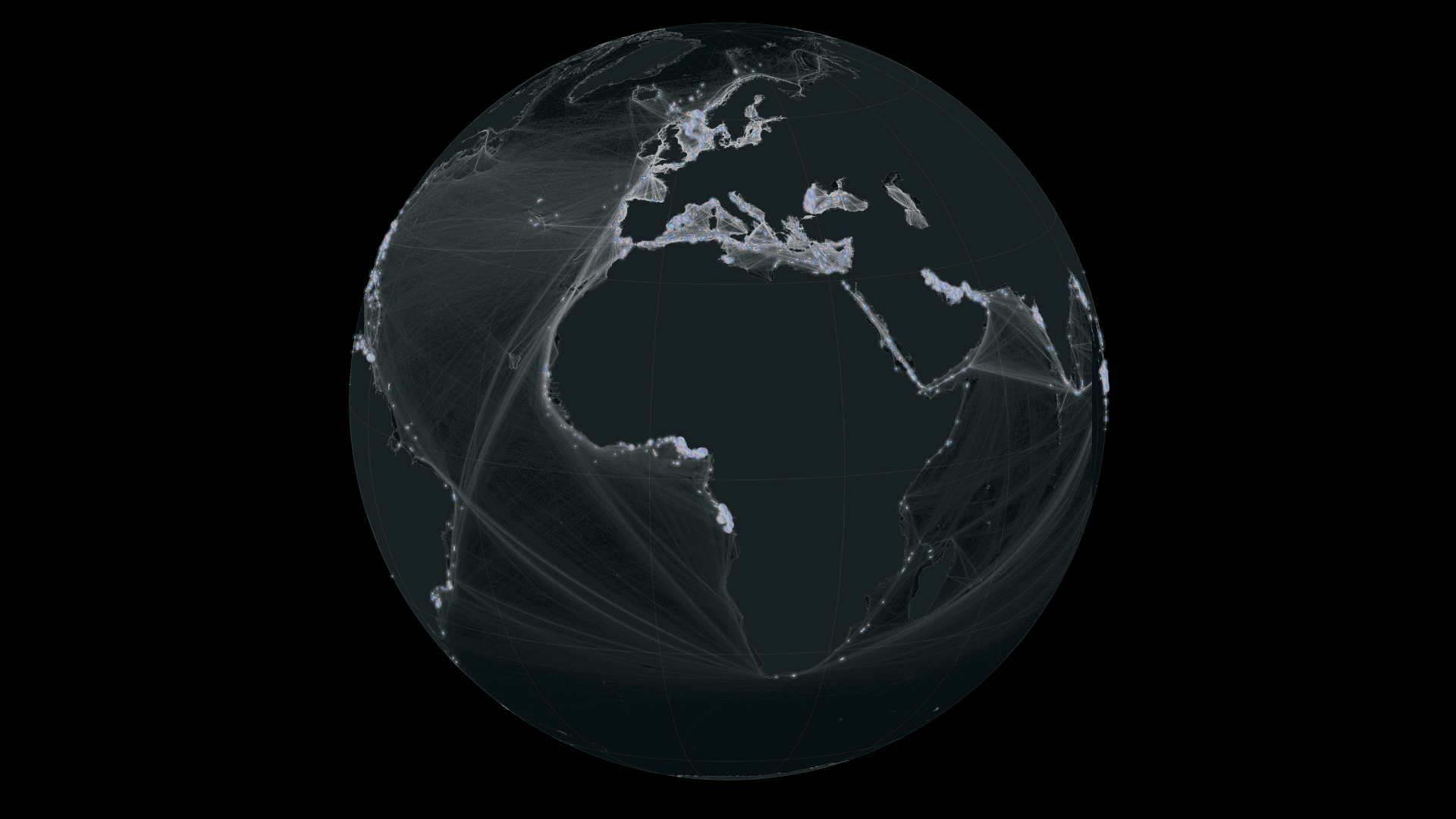
White intensity shows relative vessel activity based on AIS positions from January 2015 to February 2021. Brighter areas indicate greater activity within the dataset, bringing ports and routes across the ocean into view. The dataset includes both moving and stationary vessels, so brightness reflects activity at sea and time spent near ports. Beneath the iridescent slicks, it provides a geographic context for comparing where the two sets of records occur. World Bank / IMF · Global Shipping Traffic Density

The activity layer and slicks cover different periods. This is a long-term distribution of vessel activity, rather than vessel positions at the times of individual slick observations. Investigating a possible source requires tracks and satellite imagery matched to the observation time.

A closer look at four seas

Zooming into four seas reveals long ribbons and branching outlines. Iridescent shapes show detections from 2023–2025; white shows relative vessel activity from 2015–2021. Each arrow identifies one observation with its date and area. These different observation periods provide geographic context, rather than attribution to an individual vessel.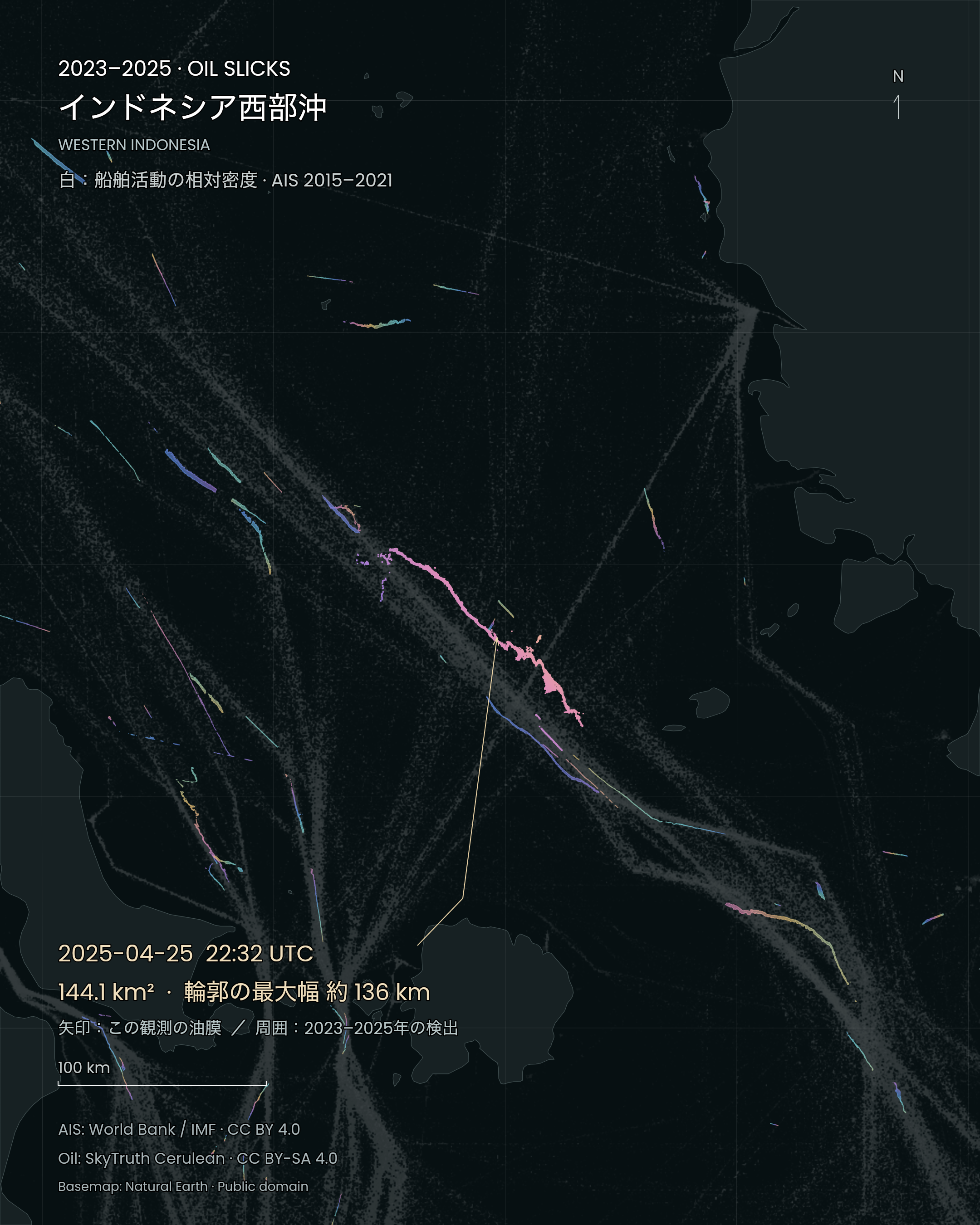

Iridescent oil-slick outlines and white vessel-activity density Off western Indonesia.

Off western Indonesia. The arrow identifies a slick observed at 2025-04-25 22:32:26 UTC: 144.1 km², approximate footprint span 136 km. Figure labels are Japanese; the date, units and geometry are shared. SORAH · SkyTruth Cerulean / World Bank / IMF / Natural Earth · CC BY-SA 4.0 · AIS: CC BY 4.0 · Natural Earth: public domain · Source · Regional projection, colour and annotations added. Iridescence does not encode thickness. Oil: 2023–2025; AIS: 2015–2021.

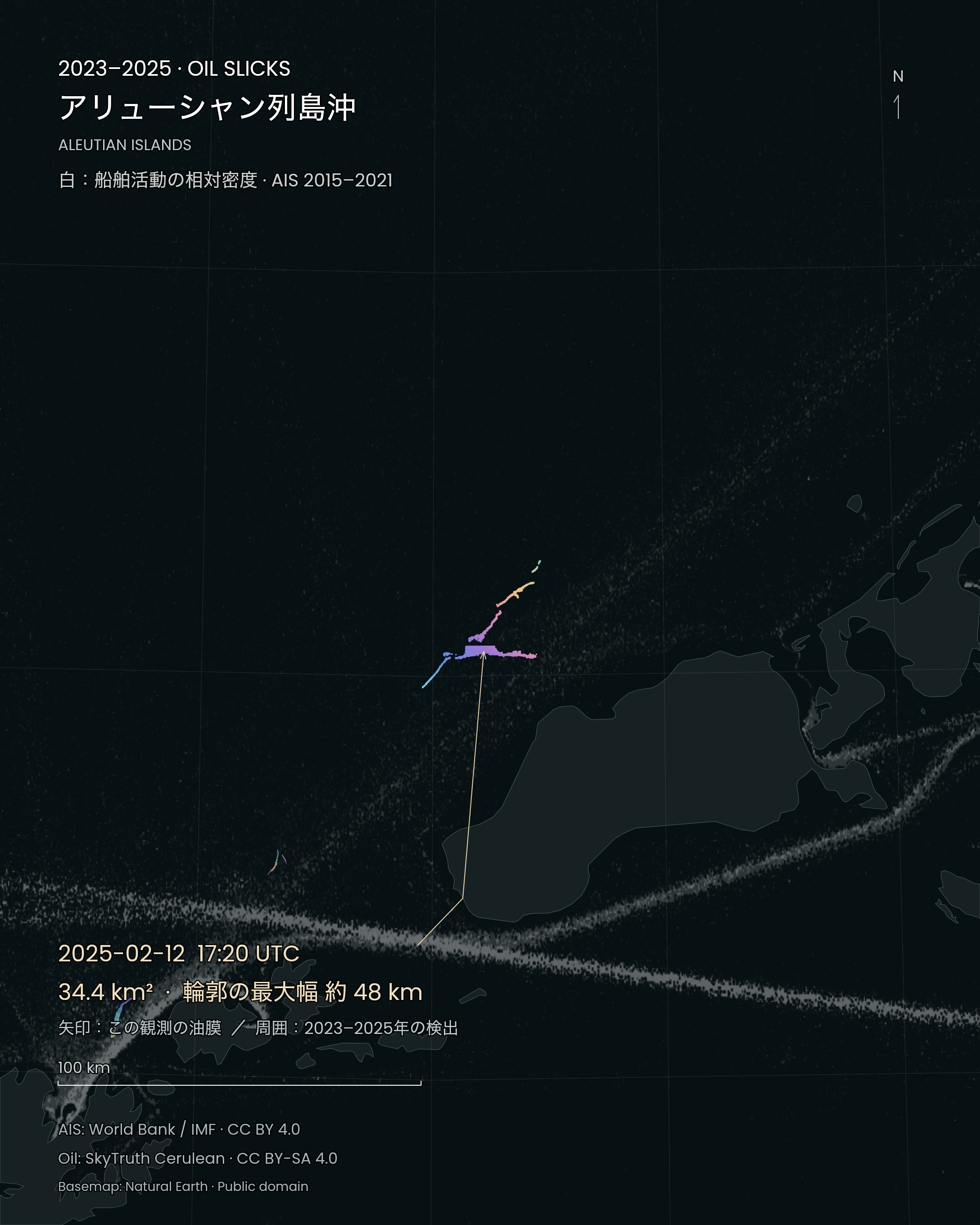
Iridescent oil-slick outlines and white vessel-activity density Near the Aleutian Islands.

Near the Aleutian Islands. The arrow identifies a slick observed at 2025-02-12 17:20:51 UTC: 34.4 km², approximate footprint span 48 km. Figure labels are Japanese; the date, units and geometry are shared. SORAH · SkyTruth Cerulean / World Bank / IMF / Natural Earth · CC BY-SA 4.0 · AIS: CC BY 4.0 · Natural Earth: public domain · Source · Regional projection, colour and annotations added. Iridescence does not encode thickness. Oil: 2023–2025; AIS: 2015–2021.

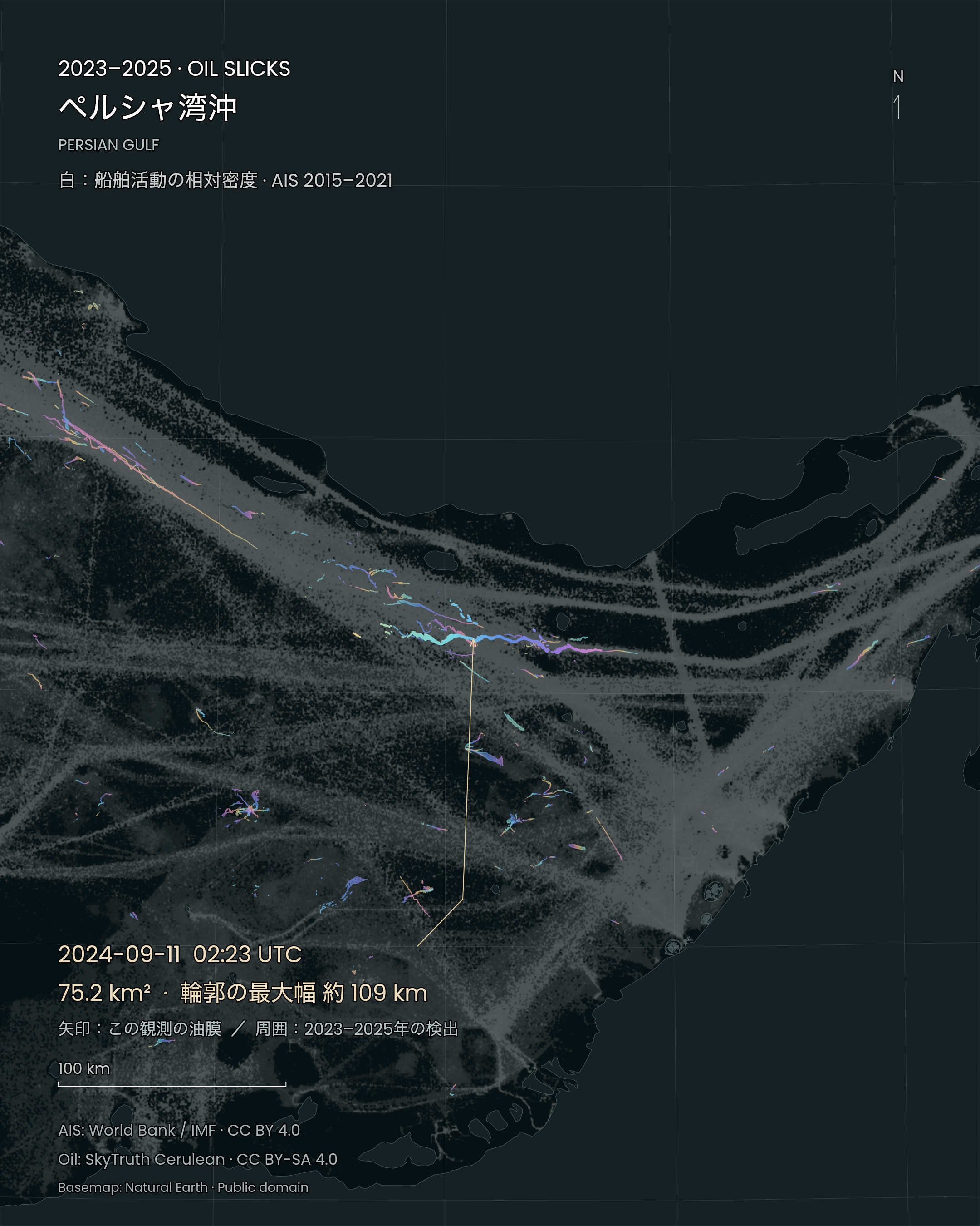
Iridescent oil-slick outlines and white vessel-activity density Persian Gulf.

Persian Gulf. The arrow identifies a slick observed at 2024-09-11 02:23:36 UTC: 75.2 km², approximate footprint span 109 km. Figure labels are Japanese; the date, units and geometry are shared. SORAH · SkyTruth Cerulean / World Bank / IMF / Natural Earth · CC BY-SA 4.0 · AIS: CC BY 4.0 · Natural Earth: public domain · Source · Regional projection, colour and annotations added. Iridescence does not encode thickness. Oil: 2023–2025; AIS: 2015–2021.

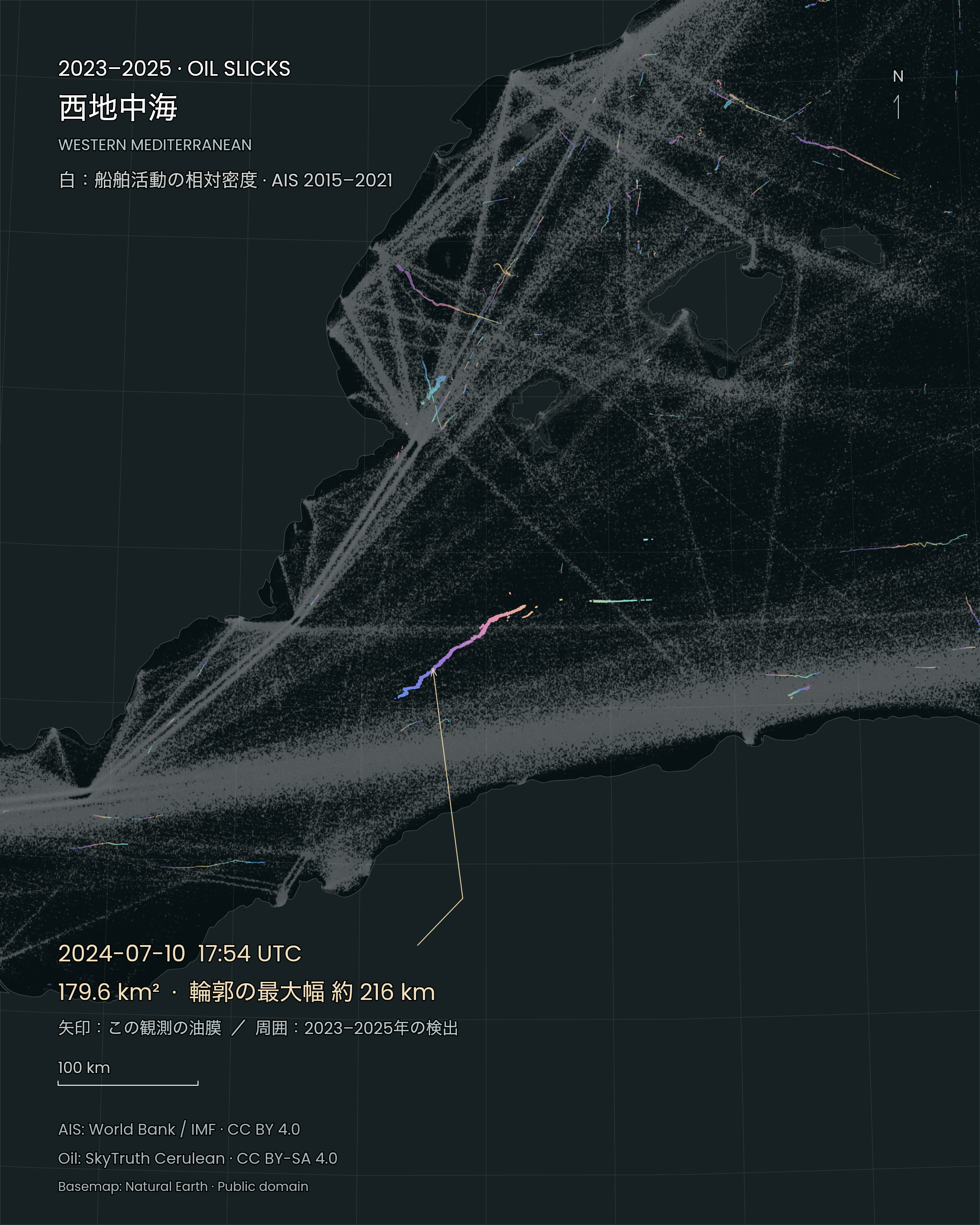
Iridescent oil-slick outlines and white vessel-activity density Western Mediterranean.

Western Mediterranean. The arrow identifies a slick observed at 2024-07-10 17:54:10 UTC: 179.6 km², approximate footprint span 216 km. Figure labels are Japanese; the date, units and geometry are shared. SORAH · SkyTruth Cerulean / World Bank / IMF / Natural Earth · CC BY-SA 4.0 · AIS: CC BY 4.0 · Natural Earth: public domain · Source · Regional projection, colour and annotations added. Iridescence does not encode thickness. Oil: 2023–2025; AIS: 2015–2021.

Radar observes the texture of the water

Synthetic aperture radar can collect observations at night and through cloud. Oil suppresses small surface waves and changes the radar response, often producing a dark shape against brighter surrounding water. Analysts then consider conditions such as weather, nearby infrastructure and vessel activity when reviewing a detection. SkyTruth · Slick details and verification

Slick verification and source attribution are separate investigative steps. Cerulean records review status for both the slick and its possible sources. A nearby vessel or structure is examined against timing and imagery when analysts assess the strength of an association. SkyTruth · Slick details and verification

In optical images, illumination can make oil appear brighter or darker than surrounding water. A NASA image from 24 May 2010 shows ribbons of oil across the Gulf of Mexico. Moving between visible-light imagery and radar observations helps explain why different kinds of evidence matter when investigating a thin layer on the sea.

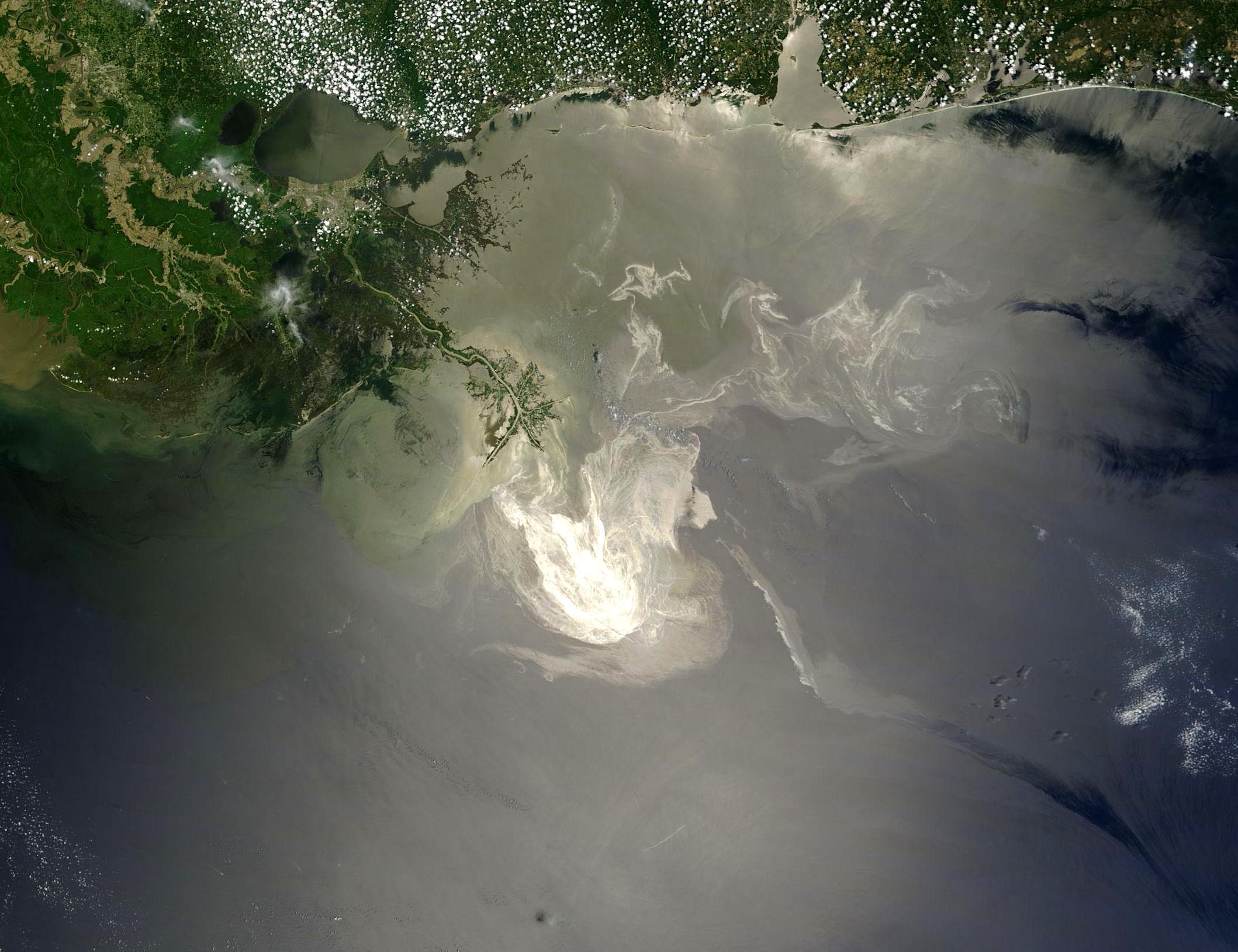
Satellite image of oil streaks offshore from the Mississippi Delta.

Oil from the Deepwater Horizon spill in the Gulf of Mexico. NASA Terra/MODIS, 24 May 2010. NASA / GSFC, MODIS Rapid Response · Public domain — NASA · Source · Supplied image unchanged; source version cropped at top and left.

What happens next depends on the oil

Oil changes after it enters the marine environment. Volatile components evaporate; waves can disperse droplets into the water; and oil mixed with water can form an emulsion that complicates removal. NOAA describes these physical, chemical and biological changes as weathering and uses knowledge of them in spill response. NOAA · Weathering processes affecting spills

Identifying the substance also matters. Light products such as gasoline or diesel have different evaporation and persistence characteristics from heavy oils. Alongside area, information on oil type, thickness and elapsed time helps responders assess conditions and plan recovery or shoreline work. An outline records a location and extent from which further investigation can proceed. NOAA · Oil types

What a thin film can mean for wildlife and coasts

Oil damages the water-repellent function of feathers and the insulation provided by mammal fur. Animals may swallow oil while grooming. Oil mixed into the water can expose fish and shellfish, affecting growth and reproduction; eggs and larvae are particularly sensitive. NOAA · Oil and marine life

Oil reaching shore can affect wetlands, tidal flats and beaches. Contaminated seafood also connects pollution with food safety and fisheries. Harm depends on the oil, amount, exposure and organisms present. Slick area alone cannot rank ecological damage. NOAA · Oil spills and coastal ecosystems

From a global map to work on a particular coast

During the Deepwater Horizon response in 2010, NOAA produced maps using satellite imagery, aerial observations and other information to describe oil locations and forecast movement. Observations preserve a position at a particular time; forecasts help people prepare for what may follow. Their distinct roles support practical decisions in the field. NOAA · Deepwater Horizon trajectory maps

A global view offers a starting point for asking where closer investigation is needed. Repeated detections or records near a coast can be examined alongside sea conditions and field evidence. Keeping the outline together with its date connects something first seen from far away to a specific body of water and the people working to understand it.

Data and representation

The selection contains 4,373 Cerulean public API records from 2023–2025 in human-reviewed anthropogenic classes 2, 4, 5, 6, 7 and 8. Annual areas sum the API’s area values after conversion to square kilometres. Repeated observations are included. Converting area to volume requires additional information, including thickness. Observation opportunities and review coverage vary; the annual increase describes this extracted set. Assessing pollution trends requires consistent observation and validation conditions. SkyTruth · Cerulean public slick data

The rotating globe displays the combined 2023–2025 detection footprints. Arrows identify large slicks using an approximate maximum span between points on the original footprint, the UTC satellite observation timestamp and an approximate location. Cyan, blue, violet, pink, gold and pale green are display colours that evoke iridescent oil sheen. The contextual satellite image records a 2010 observation and carries its own date and location.

White intensity shows relative vessel activity from World Bank / IMF Global Shipping Traffic Density, based on AIS positions from January2015–February2021, including moving and stationary vessels. Native0.005-degree values are summed by cell-centre assignment into0.1-degree cells and shown on a logarithmic scale. Absolute source magnitudes have unresolved interpretation issues, so values are not converted into vessel or passage counts. Reception and carriage biases remain; dark areas do not demonstrate the absence of ships. Six extra columns outside the longitude domain are excluded, with nonzero values and overlap discrepancies preserved in the validation record. Oil covers2023–2025; overlap does not establish a correlation coefficient or individual source. Data source: IMF’s World Seaborne Trade monitoring system (Cerdeiro et al.,2020), World Bank, CC BY4.0. World Bank / IMF · Global Shipping Traffic Density AIS raster · independent ingest audit

The globe’s pulsing glow is a display aid for locating the oil footprints. It does not represent observation time, discharge volume, movement or changing thickness.

The four regional stills use original oil polygons and the native 0.005° AIS grid, with Natural Earth 1:10m land. Map scales differ; compare annotated values when comparing areas.